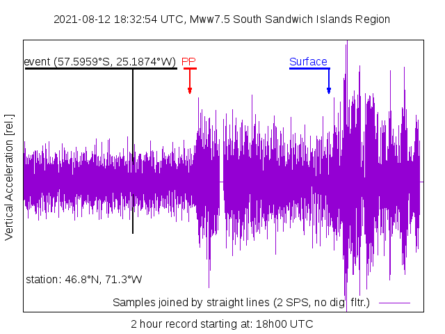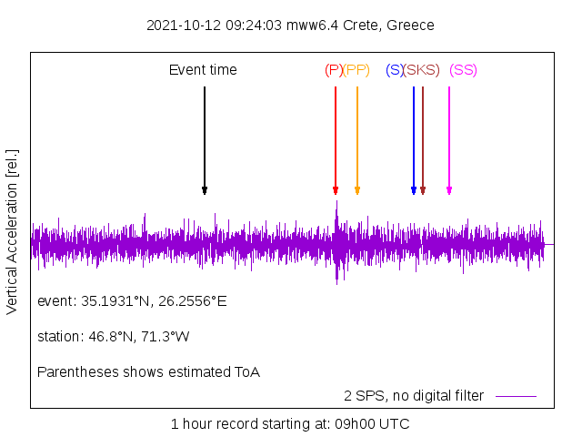
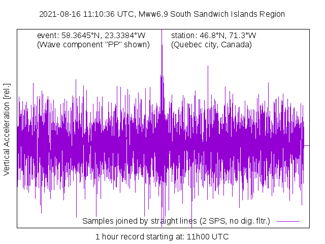
This is small signal, however the principal wave component very visible. The position of other wave components is also shown for information only.
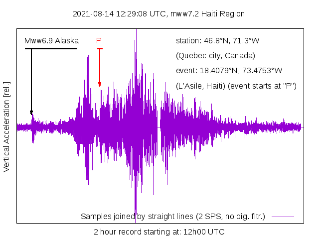
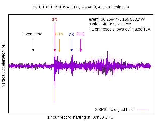
This is the first earthquake monitored from the Alaskan region.
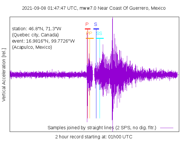
The large amplitude and moderate distance allows us to observe
more details. The arrows identified by parentheses represent the
estimated time of arrival for different propagation modes. We
think that the time coincidence and signal quality are sufficient
to identify the first two or three peaks. Please note the
background noise envelope before the first peak and later as the
signal envelope slowly decays. This shows a rather slow
dissipation of the seismic energy.
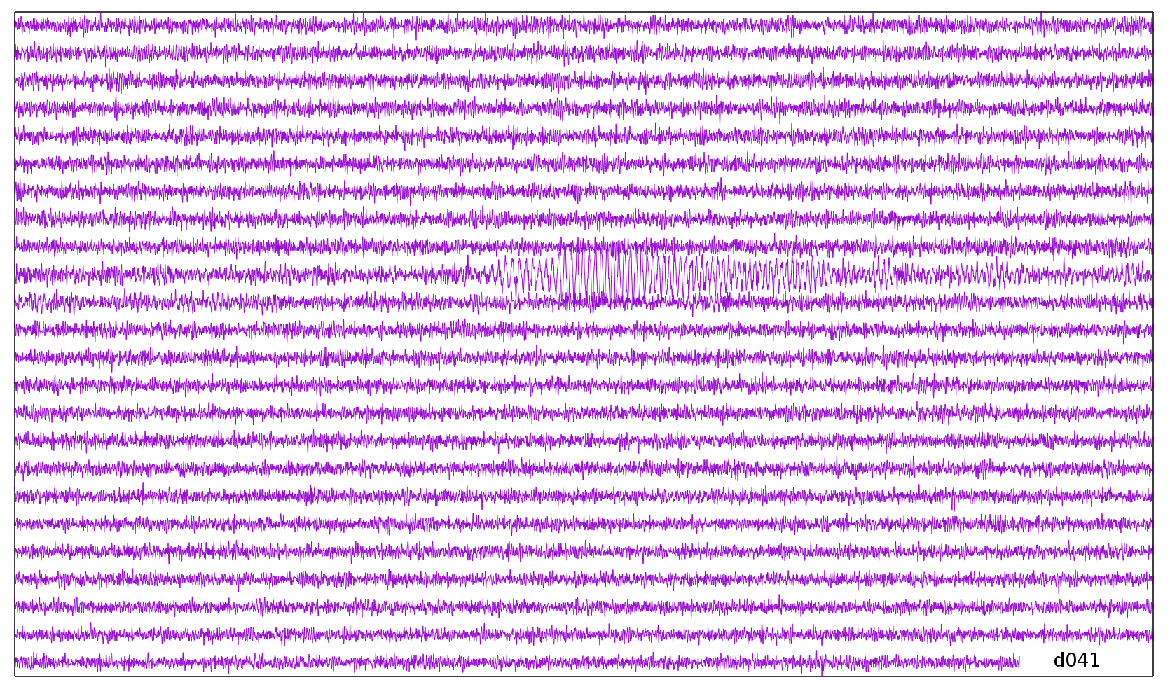
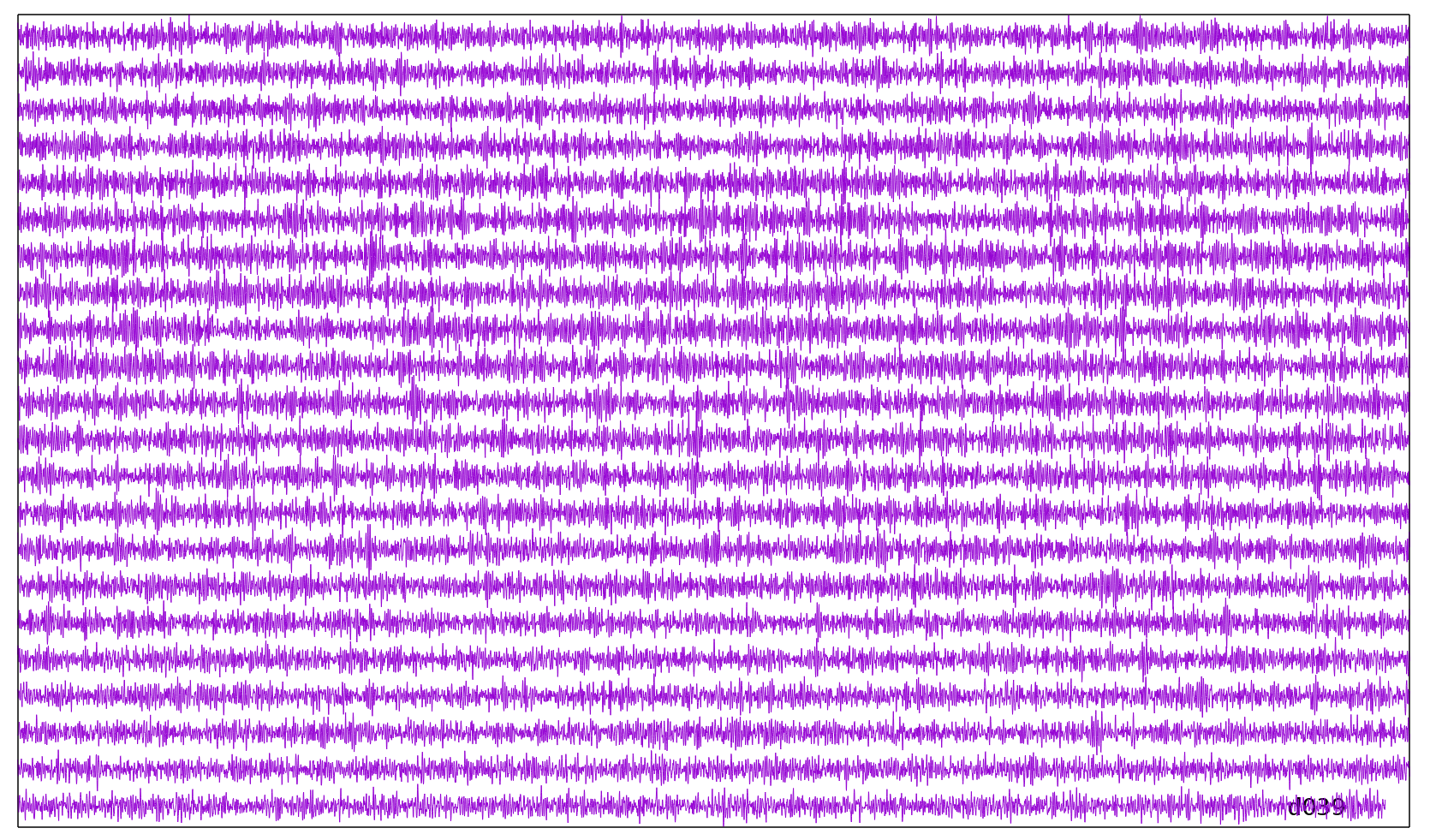
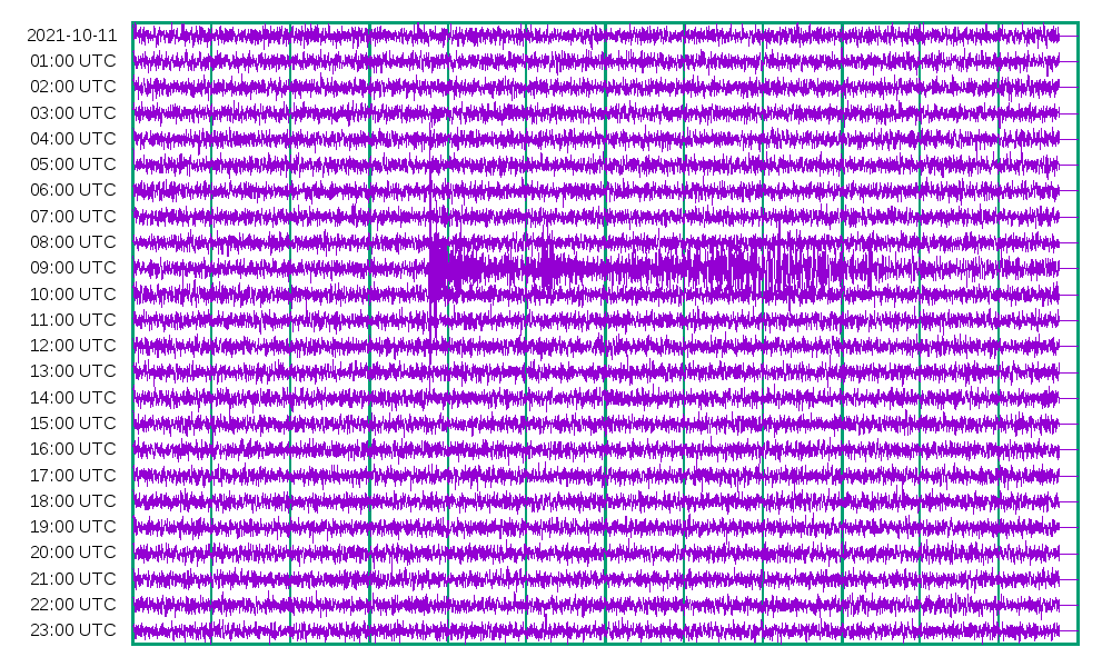
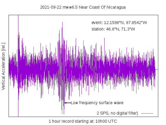
This waveform is a short segment from the larger daily plot
shown below.
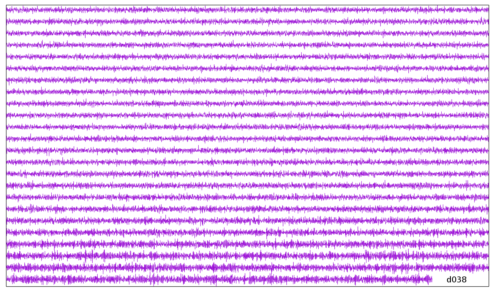
This is the weakest earthquake that I could detect.
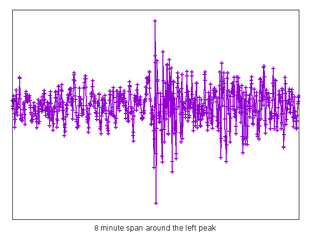
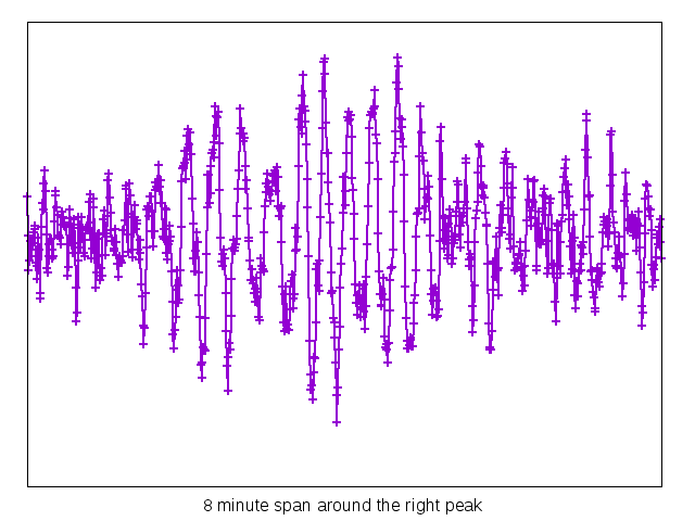
This record is a magnitude 6.5 earthquake in Nicaragua. A close look shows that the first component (bulk waves) has a higher frequency content than the second component (surface waves).
 |
 |
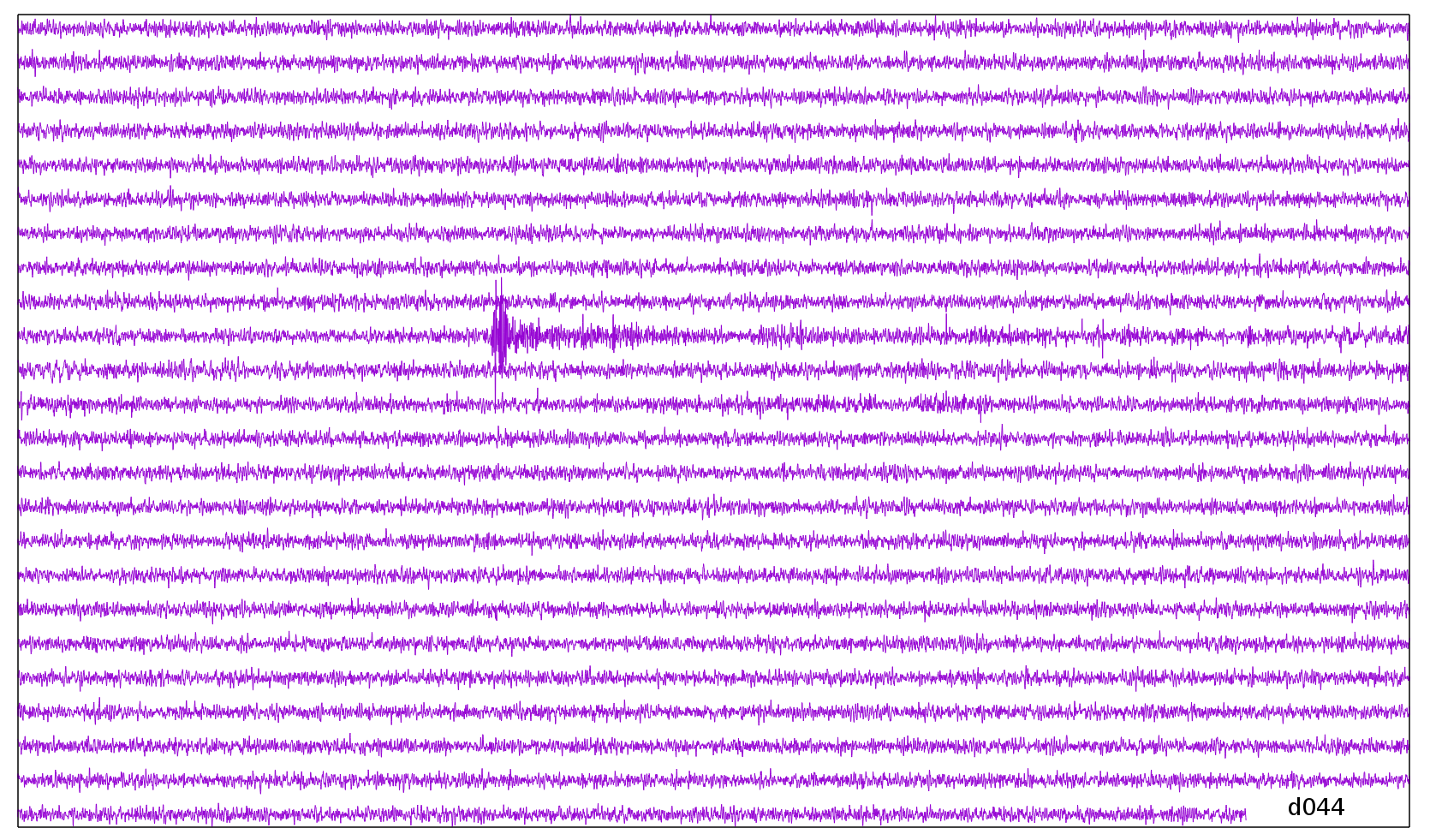
A close look on the seismograms presented earlier shows a small
dead zone in some parts of the plot. This straight line can be
interpreted as a time marker to indicate the start of the hour.
Here is an explanation.
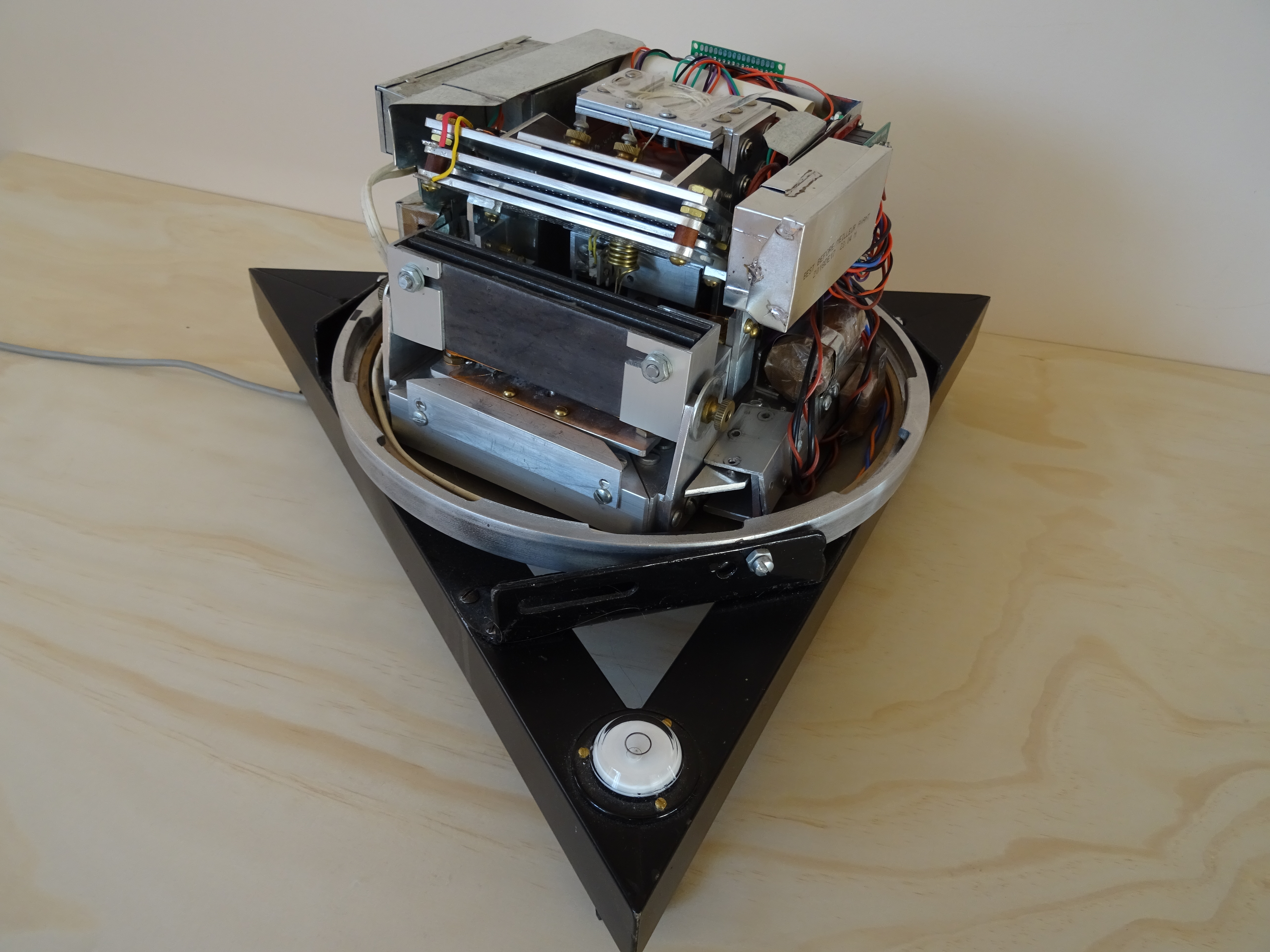
The instrument is equipped with an analog to digital converter
which is connected to a personal computer thru a USB port. The
averaging time of the converter is 0.4 second. The computer
program runs inside a loop, periodically asking for time, waiting
and then reads a number. The readings are fetched at a rate of two
samples per second. The samples are converted to floating numbers,
scaled and saved to the disk. Every file contains 7200 numbers to
cover a one hour period.
The acquisition program does not run for an infinite amount of
time. Instead it is started by the computer's job scheduler at the
beginning of the hour and stops after one hour. There is no
justification for doing this way except than saying this is still
under development, it was easy to program as opposed to a more
complex background software and finally this approach guarantees a
short down time and a fresh start in case there is a
software/computer crash. The down side to this method is we should
prevent a new job to start while the previous one has not
terminated. I wanted to avoid this dangerous situation!
Instead I run the program for a period slightly shorter than one
hour, leaving some time for the computer to terminate the
remaining conversions, close the files properly and dwell until a
new job is called. Again, this is under development and should be
improved.
The samples are stored in ASCII in the file with one number per
line. for example line number 1220 represent 10 minute and 10
second after the start of recording. The file name represent the
start time. It is easy to get a longer record by merging two or
more files together. It is then necessary to complete the
remaining of each file with dummy lines to get exactly 7200 lines.
Because this padding occurs at the end of the hour, it is easy to
write the average of the previous numbers. This is done in real
time by the acquisition program.
The whole shebang described above makes it possible/easy to
directly manipulate and plot the raw data without any further
software treatment!
There is no digital filtering applied to the samples. The analog
signal is (properly, Nyquist) filtered before conversion. This was
chosen with the objective that the raw signal is limited to
frequencies lower than one Hertz.
This one occurred in Acapulco, Mexico, but is labelled "Near
Coast of Guerrero ." I always use the same exact label supplied by
USGS WILBER to describe the events. That includes location
and time. Please see this Wikipedia page for a longer
description of the disaster.
Here is the
2021 disaster. It was located at 6 km from the town of
l'Asile in Haiti. Sadly this is the deadliest
earthquake this year with thousands casualties: Wikipedia